Matrix in R Programming: A Beginner’s Guide

You’re probably here because you opened R, saw the word matrix, and felt like the language skipped a few chapters.

That’s normal. In beginner tutorials, matrices often show up right when things start to feel more “mathy.” But a matrix in R programming is much less scary than it sounds. If you can picture a spreadsheet with rows and columns, you already understand the basic idea.

The useful part is this. Matrices help you organize numeric data in a way R can process cleanly and quickly. That matters in data science, machine learning, and even simple tasks like storing exam scores, sales numbers, pixel values, or user features for a model.

Why Your R Code Needs Matrices

A lot of beginners start with separate vectors. That works fine at first.

You might create one vector for ad spend, another for clicks, and another for conversions. Then a few days later, you’re trying to remember which value belongs to which campaign. Your code still runs, but the data starts feeling scattered.

Here’s a messy version of that setup:

ad_spend <- c(100, 150, 200)
clicks <- c(20, 35, 50)
conversions <- c(2, 4, 5)

Nothing is wrong with this. But these three vectors clearly belong together. Each position refers to the same campaign or day. When data has that kind of row-and-column structure, a matrix is often the cleaner choice.

campaign_data <- matrix(
  c(100, 150, 200,
    20, 35, 50,
    2, 4, 5),
  nrow = 3
)

campaign_data

Now your data lives in a single grid. That makes it easier to inspect, slice, and calculate with.

Why this matters for AI work

A lot of AI and machine learning prep boils down to building a feature grid. Each row might represent one customer, document, or image. Each column might represent one measured value.

That’s why matrix in r programming matters so much. It gives you a direct way to store structured numeric inputs before they go into analysis or modeling code.

Practical rule: If your data is all one type and naturally fits into rows and columns, try a matrix before reaching for something more complicated.

R’s matrix system has deep roots in the language. The matrix() function traces back to R’s early statistical-computing design in the mid-1990s, where matrices formed the backbone of core statistical functions, as described in this overview of matrices in R.

If your goal is to move from learning syntax to building actual projects, a curated list of R tools for AI deployment can help you see where matrix-based workflows fit into the bigger picture.

What Exactly Is a Matrix in R

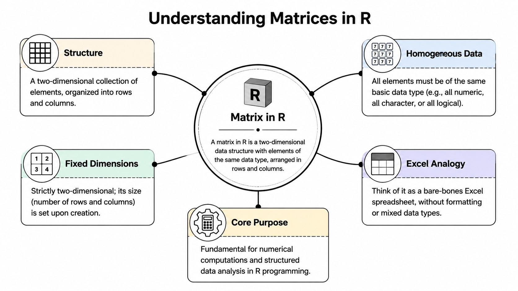
A matrix in R is a two-dimensional data structure made of rows and columns. Think of it as a stripped-down spreadsheet.

The key difference from a regular spreadsheet is that a matrix has rules. The biggest one is simple. Every cell has to hold the same kind of data.

The spreadsheet analogy that actually helps

Suppose you open Excel and create a little table:

Math	Science	English
90	85	88
78	92	81
95	89	94

That’s basically matrix-shaped data. It has rows and columns, and every value is numeric.

In R, that’s a natural fit for a matrix:

scores <- matrix(c(90, 78, 95,
                   85, 92, 89,
                   88, 81, 94), nrow = 3)

scores

What makes this powerful is that R can apply mathematical operations across the whole grid without guessing how to handle mixed content.

The homogeneity rule

Many readers often get confused. A matrix can hold numbers, or text, or logical values like TRUE and FALSE. But it can’t comfortably mix them while staying mathematically useful.

R matrices enforce homogeneity, so all elements must be the same data type. That consistency helps avoid runtime errors and unexpected conversions in model training, which matters for numerical stability and reproducibility in AI workflows, as explained in Discdown’s matrices chapter.

Here’s what happens if you mix numbers and text:

mixed_matrix <- matrix(c(1, 2, "hello", 4), nrow = 2)
mixed_matrix

R will convert everything to a common type. In this case, you’ll usually end up with character data. Beginners often expect “just one cell” to be text while the rest stay numeric. That’s not how matrices work.

A matrix is great when every box should behave the same way. That’s exactly what you want for most numeric analysis tasks.

If you’ve seen AI text workflows before, it may help to compare this with a term document matrix, which also uses a row-by-column structure to represent data in a model-friendly way.

Matrix versus data frame

Use a matrix when:

• Your values are all one type, usually numeric
• You want math operations to work naturally
• You’re preparing model input as rows and columns

Use a data frame when:

• Columns have different meanings and types
• You need names, labels, dates, categories, and numbers together
• You’re doing more general data wrangling

How to Create Matrices in R

You load a CSV for a small machine learning project, pick out the numeric columns, and now you need them in a clean row-and-column format. That is where matrices become practical. In R, a matrix is often the fastest way to turn raw values into a model-ready grid.

The main tool is matrix(). You will also use cbind() and rbind() when your data already exists in pieces.

Start with matrix()

The basic pattern looks like this:

matrix(data, nrow, ncol, byrow = FALSE)

A helpful way to read that is: “take these values and arrange them into a grid.”

Try this first:

m1 <- matrix(1:6, nrow = 2, ncol = 3)
m1

That creates a 2 by 3 matrix using the values 1 through 6.

The part that surprises many beginners is the fill direction. R fills a matrix by column unless you say otherwise. If you picture a spreadsheet, R starts with the first column, fills downward, then moves to the next column.

m1 <- matrix(1:6, nrow = 2, ncol = 3)
m1

You will get this layout:

1	3	5
2	4	6

If you want the numbers to go left to right across each row, set byrow = TRUE.

m2 <- matrix(1:6, nrow = 2, ncol = 3, byrow = TRUE)
m2

Now the layout is:

1	2	3
4	5	6

That single argument causes a lot of “oh, now I see it” moments.

Beginner tip: If your matrix should look like a table you would type by hand, use byrow = TRUE and print it right away to confirm the layout.

Build matrices from existing vectors

Sometimes your values are already sitting in separate vectors. In that case, you do not need to rebuild everything from scratch.

Use cbind() when each vector should become a column:

math <- c(90, 78, 95)
science <- c(85, 92, 89)

grades_cols <- cbind(math, science)
grades_cols

This works well for feature data. One column can be height, another can be weight, another can be age.

Use rbind() when each vector should become a row:

student1 <- c(90, 85, 88)
student2 <- c(78, 92, 81)

grades_rows <- rbind(student1, student2)
grades_rows

A simple way to remember the difference is this:

• cbind() adds columns
• rbind() adds rows

Quick comparison of creation methods

Function	What It Does	Best For
matrix()	Builds a matrix from a vector of values	Creating a matrix from scratch
cbind()	Combines objects as columns	Turning several vectors into one feature grid
rbind()	Combines objects as rows	Stacking observations or records

A realistic beginner example

Suppose you imported numeric data from a CSV and want a clean input table for a model. After reading your file with this guide to importing CSV files in R, you might pull out a few numeric columns and combine them into a matrix.

height <- c(170, 165, 180)
weight <- c(70, 60, 85)
age <- c(30, 25, 40)

features <- cbind(height, weight, age)
features

That gives you a small feature matrix. Each row represents one person. Each column represents one measured variable.

For beginner data science work, that is the point of a matrix in R. It gives you a plain numeric grid that is easy to inspect, easy to combine, and ready for analysis.

Manipulating and Naming Matrix Data

Creating a matrix is step one. The key “aha” moment usually happens when you start pulling values out of it.

In R, matrix access uses square brackets with this pattern:

my_matrix[row, column]

That means you always think in two directions at once. First row, then column.

Start with a small 3 by 3 matrix

m <- matrix(1:9, nrow = 3, byrow = TRUE)
m

That gives you:

1	2	3
4	5	6
7	8	9

Now let’s pull things out.

Get one value

m[2, 3]

This means row 2, column 3. The result is 6.

Get a whole row

m[2, ]

Leave the column spot blank, and R returns the whole second row.

Get a whole column

m[, 1]

Leave the row spot blank, and R returns the whole first column.

Get a smaller block

m[1:2, 2:3]

That grabs rows 1 through 2 and columns 2 through 3.

When matrix indexing feels confusing, read it out loud. “Rows first, columns second.” That tiny habit fixes a lot of beginner mistakes.

Naming rows and columns

Unnamed matrices work, but named matrices are much easier to read.

scores <- matrix(c(90, 85, 88,
                   78, 92, 81,
                   95, 89, 94),
                 nrow = 3, byrow = TRUE)

rownames(scores) <- c("Alex", "Jordan", "Sam")
colnames(scores) <- c("Math", "Science", "English")

scores

Now the matrix looks more like real data instead of a mystery grid.

Once names exist, your indexing becomes more human-readable:

scores["Jordan", "Science"]
scores[, "Math"]
scores["Alex", ]

Editing values inside a matrix

You can also change entries directly:

scores[1, 1] <- 91
scores

Or update a whole column:

scores[, "English"] <- c(89, 82, 95)
scores

This is one reason matrices stay useful in data prep. You can build a numeric grid with cbind() and then clean or adjust values using indexing.

Key Matrix Functions for Data Analysis

A matrix becomes really useful once you start asking questions of it.

If you treat a matrix like a numeric spreadsheet, these functions are the tools you reach for to check its size, rotate it, summarize it, and do the kind of math that shows up in model prep.

Check shape with dim()

Before you run calculations, check the shape of your matrix. This helps you catch mistakes early, especially when you are preparing features for a machine learning model.

m <- matrix(1:12, nrow = 3, byrow = TRUE)
dim(m)

R returns 3 4, which means 3 rows and 4 columns.

A simple habit helps here. Read dim(m) as, “How many spreadsheet rows and columns do I have?” If a model expects one shape and your matrix has another, this is often the first clue that something is off.

Transpose with t()

t() flips the grid. Rows become columns, and columns become rows.

m <- matrix(1:6, nrow = 2, byrow = TRUE)
m
t(m)

This comes up often in data prep. You may collect data one way, then need to turn it so each row represents one observation and each column represents one feature. That kind of cleanup shows up in many beginner projects, including k-nearest neighbor in R examples.

Element-wise multiplication versus matrix multiplication

Beginners mix these up all the time because both use multiplication symbols, but they do different jobs.

* multiplies cell by cell.
%*% performs matrix multiplication.

a <- matrix(c(1, 2, 3, 4), nrow = 2)
b <- matrix(c(5, 6, 7, 8), nrow = 2)

a * b

That code matches each position in a with the same position in b.

a %*% b

This second version follows matrix multiplication rules. It combines rows from the first matrix with columns from the second. If that sounds abstract, use a spreadsheet picture in your head. Cell-by-cell multiplication edits matching boxes. Matrix multiplication combines full rows and columns to create new values.

That difference matters in AI work. Cell-by-cell math is common in feature scaling and transformations. Matrix multiplication appears under the hood in many modeling methods discussed in AI and machine learning trends for 2026.

Work across rows or columns with apply()

apply() helps you run the same calculation across each row or each column without writing a loop.

scores <- matrix(c(90, 85, 88,
                   78, 92, 81,
                   95, 89, 94),
                 nrow = 3, byrow = TRUE)

apply(scores, 1, mean)

The 1 means “work across rows,” so R gives you one mean for each row.

apply(scores, 2, mean)

The 2 means “work across columns,” so R gives you one mean for each column.

This is handy for quick summaries. You can get student averages, feature means, row totals, or column maximums with the same basic pattern.

Other handy tools

A few small functions save time:

• diag() gets the diagonal values of a matrix, or creates a diagonal matrix.
• solve() computes a matrix inverse in cases where inversion is possible.
• is.matrix() checks whether an object is a matrix.

m <- matrix(c(1, 2, 3, 4), nrow = 2)

diag(m)
is.matrix(m)

You do not need to master every matrix function at once. Start with dim(), t(), *, %*%, and apply(). Those five cover a large share of the matrix work beginners do in real data analysis.

Matrix Performance in Machine Learning

When people say matrices are better for numeric work in R, they don’t just mean “tidier.” They mean faster and more suitable for heavy calculations.

That matters when you’re building models, transforming features, or running repeated operations across large numeric datasets.

Why matrices often beat data frames

Matrices in R are optimized for numeric computation and are significantly faster than data frames for large numeric work because R stores them in column-major order and can use low-level BLAS optimizations for operators like %*%, according to this R-Bloggers explanation of matrices.

The plain-English version is simple. A matrix gives R a more predictable structure. Every cell is the same type, and the data lives in memory in a way that makes math easier to execute efficiently.

For machine learning, that fits the job well. A model usually wants clean numeric input, not a flexible table full of mixed types.

What this looks like in practice

Suppose you’re building a k-nearest neighbors classifier. You want a numeric feature grid, not a mixed object with text labels mixed into your calculation columns. A tutorial on k-nearest neighbor in R makes a lot more sense once you’re comfortable separating model features into matrix-friendly form.

Here’s a basic example:

features <- matrix(c(
  170, 70, 30,
  165, 60, 25,
  180, 85, 40
), nrow = 3, byrow = TRUE)

new_case <- matrix(c(175, 75, 32), nrow = 1)

features
new_case

That’s the kind of structure many algorithms expect under the hood.

A note on sparse data

Some AI problems produce huge grids with lots of zeros. Text classification is a classic example. Recommendation systems can look similar too.

In those cases, people often move from base matrices to sparse matrices, especially through tools like the Matrix package. If you’re trying to connect beginner R skills to the bigger direction of modern AI work, this guide to AI and machine learning trends for 2026 offers a useful broad view of where efficient data structures fit.

Working opinion: For beginner ML in R, learn the regular matrix first. Once that feels natural, sparse matrices become much easier to understand.

R Matrix FAQ and Common Errors

Why did my numeric matrix turn into text

Because matrices must hold one data type. If you mix numbers and strings, R usually converts everything to character so the matrix stays homogeneous.

matrix(c(1, 2, "x", 4), nrow = 2)

If you need mixed columns, use a data frame instead.

What’s the difference between * and %*%

* means element-wise multiplication. %*% means matrix multiplication.

a <- matrix(c(1, 2, 3, 4), nrow = 2)
b <- matrix(c(5, 6, 7, 8), nrow = 2)

a * b
a %*% b

If your result looks strange, this is often the reason.

How do I convert a data frame to a matrix

Use as.matrix().

df <- data.frame(x = c(1, 2), y = c(3, 4))
as.matrix(df)

Do this when your data frame contains values that should become a uniform grid for numeric work. If the data frame contains mixed types, R may coerce everything to a common type, so check the result.

---

If you’re learning R for AI, data science, or practical model building, YourAI2Day is a solid place to keep going. It brings together AI news, tools, and beginner-friendly explainers that can help you connect core concepts like matrices to real-world workflows.