Merge Data Frames R: Master Your Joins

You’ve got two files open. One has customer orders. The other has customer details. A third has support tickets. A fourth has model features exported from another team’s pipeline. None of them are useful enough on their own.

That’s usually the moment people search for merge data frames r.

The good news is that R gives you several solid ways to combine datasets. The bad news is that the easy examples you see in many tutorials don’t prepare you for the messy version of this task. Real data has duplicate keys, missing values, mismatched column names, and row counts that suddenly explode after a join.

I’ve been there. The same confusion points often arise: “Why did my rows multiply?”, “Why did records disappear?”, “Why is this so slow?”, and “Why are my IDs not matching when they look identical?” Those are normal questions. The skill isn’t just knowing the syntax. It’s learning how to merge with confidence, check your work, and choose the right tool when the data gets large.

Why Merging Data Frames is Your Data Science Superpower

A lot of useful analysis starts with an incomplete table.

Maybe you have ecommerce transactions in one CSV, marketing campaign metadata in another, and user profile data in a third. You can’t answer “Which customer segment responds best to discount emails?” until those datasets live together in one analysis-ready table. The same thing happens in machine learning. Feature engineering often means pulling signals from multiple sources, then joining them into a single training set.

That’s why merging is such a foundational skill. You’re not just combining spreadsheets. You’re building context.

One practical example

Say you have these two datasets:

• orders with customer_id, order_id, and total_spend
• customers with customer_id, city, and signup_date

On their own, they answer separate questions. Together, they let you ask better ones:

• Which cities generate the highest-value orders?
• Do newer customers spend differently from long-time customers?
• Are there customer IDs in sales data that don’t exist in the CRM?

That last question matters more than beginners expect. In many AI workflows, bad joins create quiet data quality problems. The model still trains. The dashboard still renders. But the underlying table is wrong.

Practical rule: Treat every merge as a data quality step, not just a coding step.

You’ll also run into a second reality quickly. Sometimes your original data isn’t enough, so teams enrich it with outside attributes such as company, demographic, or location signals. If you’re looking into that side of the workflow, this roundup of RevoScale details top enrichment tools is a useful companion because enrichment only becomes valuable after you can join the added fields cleanly.

Before you merge anything, it also helps to make sure you imported the raw files correctly. If column types came in wrong, your join can fail for reasons that seem mysterious until you inspect the import step. A basic cleanup pass often starts with reliable CSV loading, and this guide on importing CSV files in R is worth keeping nearby.

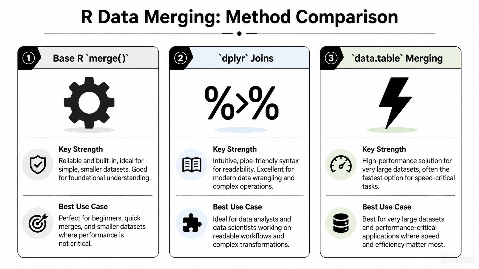
The three ways most people do this in R

R gives you a few main paths:

1. Base R merge() for built-in, dependency-free joins
2. dplyr joins for clearer, modern syntax
3. data.table and SQL-style options when performance or query style matters

Each has a place. The trick is matching the tool to the job, then validating that the merge did what you intended.

The Classic Approach Merging with Base R

Base R’s merge() is old, stable, and still worth learning. The merge() function has been part of core R since the language’s initial release in 1997, performs an inner join by default, and remains common in beginner workflows because it has no dependencies, with the function documented in R’s official materials in the base R merge documentation.

Start with two small tables

Let’s use a simple example you can run exactly as written.

orders <- data.frame(
  customer_id = c(101, 102, 103, 105),
  order_total = c(120, 85, 200, 60)
)

customers <- data.frame(
  customer_id = c(101, 102, 104, 105),
  customer_name = c("Ana", "Ben", "Chris", "Dina"),
  city = c("Austin", "Boston", "Chicago", "Denver")
)

The shared key is customer_id. That’s the column R can use to line up rows.

Inner join with merge()

The default behavior keeps only rows that match in both data frames.

merge(orders, customers, by = "customer_id")

You’ll get rows for 101, 102, and 105. You won’t get 103 because it exists only in orders, and you won’t get 104 because it exists only in customers.

That’s an inner join.

The arguments that matter most

The usual syntax is:

merge(x, y, by, by.x, by.y, sort = TRUE)

Here’s what to focus on:

• x and y are the two data frames
• by names the shared key if both tables use the same column name
• by.x and by.y let you match different column names
• sort = TRUE sorts by the join column unless you turn it off

If the key column names differ, do this:

customers2 <- data.frame(
  id = c(101, 102, 104, 105),
  customer_name = c("Ana", "Ben", "Chris", "Dina")
)

merge(orders, customers2, by.x = "customer_id", by.y = "id")

That’s one of those “I wish I knew this sooner” arguments. New users often rename columns manually when they don’t have to.

Left, right, and full joins

The merge() function feels less obvious than dplyr, but it’s still straightforward once you know the flags.

Left join

Keep all rows from the first data frame.

merge(orders, customers, by = "customer_id", all.x = TRUE)

You’ll keep 103 from orders, and the customer columns for that row will be NA.

Right join

Keep all rows from the second data frame.

merge(orders, customers, by = "customer_id", all.y = TRUE)

Now 104 appears, with missing order information.

Full outer join

Keep everything from both tables.

merge(orders, customers, by = "customer_id", all = TRUE)

This is useful when you want the full union and plan to inspect unmatched records.

If you’re ever unsure which join you just did, inspect the row count and the unmatched IDs immediately. Most merge mistakes look harmless at first.

What happens with duplicate column names

Suppose both tables have a column called status, but you’re joining on customer_id.

orders$status <- c("paid", "paid", "refunded", "paid")
customers$status <- c("active", "active", "inactive", "active")

merged_df <- merge(orders, customers, by = "customer_id")

R will keep both status columns and rename them with suffixes like .x and .y.

That means:

• status.x came from the first data frame
• status.y came from the second data frame

This is helpful, but it can also make a messy result if you didn’t realize both tables had overlapping field names. Always scan the output column names after a merge.

A few base R habits that save time

Here’s a short checklist I still use:

• Check the key first: str(orders$customer_id) and str(customers$customer_id) should be compatible.
• Turn off sorting if order matters: use sort = FALSE.
• Expect row multiplication if keys repeat: merge() creates all possible pairs when there are multiple matches.
• Be explicit when names differ: use by.x and by.y instead of renaming columns in a rush.

When base R is the right choice

Base R is a good fit when:

Situation	Why merge() works well
You want no extra packages	It’s already available
You’re teaching or learning joins	The mechanics are easy to see
You need reproducible scripts in minimal environments	No dependency setup
You have moderate-sized data	It handles common workloads cleanly

It may not be the prettiest syntax, but it’s dependable. And once you understand merge(), every other join style in R starts to make more sense.

Modern and Readable Joins with dplyr

If merge() feels a little mechanical, dplyr usually feels more natural. The package introduced SQL-like join verbs such as inner_join() and left_join(), and by 2024 the tidyverse suite had over 10 million downloads, with reporting that dplyr joins are about 20% faster than base merge for many common operations and that they’re widely used in modern data science workflows in InfoWorld’s discussion of merge methods in R.

The biggest advantage is readability

With dplyr, the function name says what the join does. You don’t have to remember whether all.x = TRUE means left join. The name tells you directly.

Using the same sample data:

library(dplyr)

orders <- data.frame(
  customer_id = c(101, 102, 103, 105),
  order_total = c(120, 85, 200, 60)
)

customers <- data.frame(
  customer_id = c(101, 102, 104, 105),
  customer_name = c("Ana", "Ben", "Chris", "Dina"),
  city = c("Austin", "Boston", "Chicago", "Denver")
)

Now the joins become self-documenting.

inner_join(orders, customers, by = "customer_id")
left_join(orders, customers, by = "customer_id")
right_join(orders, customers, by = "customer_id")
full_join(orders, customers, by = "customer_id")

That’s one reason many analysts stick with dplyr for daily work. The code is easier to scan later, especially in long pipelines.

Different key names are cleaner too

When the key names don’t match, dplyr handles it clearly.

customers2 <- data.frame(
  id = c(101, 102, 104, 105),
  customer_name = c("Ana", "Ben", "Chris", "Dina")
)

left_join(orders, customers2, by = c("customer_id" = "id"))

That line is easy to read: match orders$customer_id to customers2$id.

If you’ve seen newer syntax using join_by(), it can make intent even clearer:

left_join(orders, customers2, by = join_by(customer_id == id))

Why beginners get less lost with dplyr

The verbs reduce cognitive load. You don’t spend as much mental energy decoding arguments, so you can focus on the data itself.

That matters when your join is part of a longer workflow:

orders %>%
  left_join(customers, by = "customer_id") %>%
  filter(order_total > 80)

This style reads top to bottom like a sequence of actions.

The joins many tutorials skip

A big gap in beginner content is filtering joins. These don’t add columns. They help you answer “which rows match?” and “which rows failed to match?”

semi_join()

Keeps rows from the first table that have a match in the second.

semi_join(orders, customers, by = "customer_id")

You’ll get orders for IDs 101, 102, and 105, but no new customer columns are added.

anti_join()

Keeps rows from the first table that do not have a match in the second.

anti_join(orders, customers, by = "customer_id")

You’ll get the row for 103.

That makes anti_join() one of the best debugging tools in R.

Diagnostic shortcut: After an inner join, run an anti_join() on the original left table. It shows exactly what got dropped.

Here’s a short walkthrough if you want to see the workflow explained visually:

A realistic debugging pattern

This pattern saves a lot of time:

joined <- left_join(orders, customers, by = "customer_id")

missing_customers <- anti_join(orders, customers, by = "customer_id")
missing_orders <- anti_join(customers, orders, by = "customer_id")

Now you know:

• which orders didn’t find customer records
• which customer records have no matching orders

That’s more useful than staring at NA values and guessing what happened.

When dplyr is the right default

I usually recommend dplyr when:

• You care about readability: teammates can understand the join quickly.
• You’re already using tidyverse tools: it fits naturally with filter(), mutate(), and summarise().
• You want better debugging flow: anti_join() and semi_join() are handy.
• Your data is medium to large, but not pushing your machine to its limits: performance is often solid.

dplyr won’t solve every scaling problem, but for many analysts it hits the sweet spot between clarity and speed.

High-Performance Merging with data.table and sqldf

Once your joins start hitting millions of rows, you stop caring only about syntax. You care about memory, elapsed time, and whether your laptop sounds like it’s preparing for takeoff.

That’s where data.table earns its reputation. And if you think naturally in SQL, sqldf can be a comfortable bridge.

data.table for speed-first workflows

The appeal of data.table is simple. It’s built for large data work and efficient operations.

A basic setup looks like this:

library(data.table)

orders_dt <- data.table(
  customer_id = c(101, 102, 103, 105),
  order_total = c(120, 85, 200, 60)
)

customers_dt <- data.table(
  customer_id = c(101, 102, 104, 105),
  customer_name = c("Ana", "Ben", "Chris", "Dina")
)

Set keys if you want repeated joins on the same column:

setkey(orders_dt, customer_id)
setkey(customers_dt, customer_id)

Then join:

orders_dt[customers_dt]

Or more explicitly:

customers_dt[orders_dt, on = .(customer_id)]

That syntax throws people at first. The trick is to read it as “take customers_dt, line it up to orders_dt, matching on customer_id.”

Why people switch to data.table

Three reasons come up again and again:

• Large joins finish faster
• Memory behavior is often better
• Repeated production joins become less painful

If your AI workflow builds training data from many sources, the performance difference becomes practical, not academic.

On large datasets, a slower join doesn’t just waste time. It slows experimentation, debugging, and model iteration.

A SQL option with sqldf

Some analysts don’t want new R-native syntax. They want SQL.

That’s where sqldf can help:

library(sqldf)

sqldf("
  SELECT o.customer_id, o.order_total, c.customer_name
  FROM orders o
  INNER JOIN customers c
    ON o.customer_id = c.customer_id
")

If you already understand SQL joins, this can feel very natural.

It also connects neatly with broader SQL learning. If joins, grouping, and aggregation are part of the same workflow for you, this refresher on what GROUP BY does in SQL fits well alongside SQL-based merging in R.

When to use which

Here’s the simplest rule of thumb:

Tool	Best fit
data.table	Very large datasets, speed-sensitive pipelines, repeated joins
sqldf	Analysts who already think in SQL and want familiar syntax
Base R or dplyr	General-purpose work where readability is a bigger concern

One caution most merge tutorials skip

A lot of tutorials focus on syntax and join types, but they don’t spend much time on scaling behavior. That leaves a gap for people working on enterprise or AI pipelines where merges are often one of the more expensive steps.

If your data is getting large enough that merges feel slow, that’s your signal to benchmark rather than guess. Sometimes a cleaner-looking solution is fine. Sometimes you need a speed-first tool.

Handling Real-World Merge Scenarios and Problems

Merge tutorials usually get too polite, assuming your keys are clean, unique, typed correctly, and present in both files.

Real data rarely behaves that well.

For multi-key joins and large merge workflows, one reported analysis notes that 35% of merge errors stem from non-unique keys causing row duplication, while 28% come from heavy NA output in outer joins, with guidance such as checking duplicates and using sort = FALSE when row order matters in this discussion of multi-key merge pitfalls.

Merging on multiple keys

Sometimes one column isn’t enough. Maybe id repeats every year, so the true key is id + year.

In base R:

sales <- data.frame(
  id = c(1, 1, 2),
  year = c(2023, 2024, 2024),
  revenue = c(500, 550, 700)
)

targets <- data.frame(
  id = c(1, 1, 2),
  year = c(2023, 2024, 2024),
  target = c(480, 600, 650)
)

merge(sales, targets, by = c("id", "year"), all.x = TRUE, sort = FALSE)

In dplyr:

left_join(sales, targets, by = c("id", "year"))

That’s the easy part. The hard part is making sure those keys are unique.

Duplicate keys are the silent row multiplier

This is one of the most common surprises in merge data frames r work. You expected one row per customer. You got three rows per customer. That’s usually because one or both tables have duplicate keys.

Check before you join.

duplicated(customers$customer_id)
customers[duplicated(customers$customer_id), ]

For a composite key:

duplicated(paste(targets$id, targets$year))
targets[duplicated(paste(targets$id, targets$year)), ]

If duplicates exist, your join may create all combinations of matches. That’s correct behavior from R. It’s just often not what you intended.

What to do about duplicates

• If duplicates are invalid: clean them before merging.
• If duplicates are expected: aggregate first so each key becomes unique.
• If duplicates carry meaning: accept the row multiplication, but do it knowingly.

Here’s an aggregation example:

library(dplyr)

customers_clean <- customers_raw %>%
  group_by(customer_id) %>%
  summarise(last_signup = max(signup_date), .groups = "drop")

Now the key is unique again.

Never assume a business ID is unique because someone told you it is. Check it.

NA values and mismatched types

A join can also fail because the key columns don’t have the same type.

One table has character ZIP codes like "02110". The other has numeric values like 2110. They may look similar when printed, but they won’t join correctly without cleanup.

str(df1$zip)
str(df2$zip)

If needed:

df2$zip <- as.character(df2$zip)

NA values create their own confusion. In full joins, you can end up with a lot of missing fields and lose track of what matched and what didn’t.

A simple cleanup pattern is:

merged <- merge(df1, df2, by = "id", all = TRUE)
bad_rows <- merged[!complete.cases(merged), ]

That won’t fix the problem for you, but it gives you a focused set of rows to inspect.

Validating the merge instead of trusting it

A good merge isn’t just code that runs. It’s code that produces the right table.

I usually validate in three quick ways:

1. Check row counts before and after
2. Inspect unmatched records
3. Spot-check a few key IDs manually

In dplyr:

joined <- left_join(orders, customers, by = "customer_id")

anti_join(orders, customers, by = "customer_id")
anti_join(customers, orders, by = "customer_id")

In base R, a rough unmatched check can look like this:

orders[!(orders$customer_id %in% customers$customer_id), ]
customers[!(customers$customer_id %in% orders$customer_id), ]

That’s not as elegant as anti_join(), but it works.

Mismatched names and mapped domains

Merges get even more delicate when the data comes from heavily structured domains like healthcare. Column names might differ, source systems may encode concepts differently, and “same field” can mean “same idea, different representation.”

If you work in that kind of environment, these strategies for mapping healthcare data are useful because they show why joining is often only half the problem. Field alignment and concept mapping matter just as much.

And if your merge is part of a broader model-building workflow, this guide on data preparation for machine learning is a helpful next step because joins, missing values, and feature consistency tend to show up together.

A practical troubleshooting checklist

When a merge looks wrong, run this list in order:

• Check key types: character vs numeric mismatches are common.
• Check uniqueness: duplicates often explain row explosions.
• Check unmatched rows: use anti_join() or %in%.
• Check row order assumptions: some joins reorder rows unless you control for it.
• Check suffix columns: .x and .y may reveal overlapping fields you forgot about.
• Check a tiny sample manually: five hand-verified rows can reveal the whole issue.

That habit will save you hours. It also builds trust in your pipeline, which matters a lot once merged data feeds dashboards or models.

Choosing Your Method and a Look at Performance

Most merge tutorials stop once the code works. That’s not enough if you’re working with larger datasets, shared pipelines, or AI workflows where data prep runs repeatedly.

One of the biggest gaps in existing content is scalability. A recurring complaint in the R ecosystem is that tutorials explain syntax but don’t explain how merge(), dplyr, and data.table behave as data grows, especially when you need to think about memory use and computation time as noted in this discussion about the scalability gap in merge tutorials.

A decision framework that works in practice

You don’t need one “best” tool. You need the right one for the current job.

Use base R when simplicity matters

Choose merge() when:

• you want no package dependency
• you’re writing a small script
• you need to teach or understand the mechanics clearly
• your data size is manageable

It’s especially good for learning because it forces you to think carefully about join behavior.

Use dplyr when readability matters

Choose dplyr when:

• you already use pipes
• your workflow includes mutate(), filter(), and summarise()
• teammates need to read your code later
• debugging unmatched rows is part of the job

In everyday analytics work, this is often the best default.

Use data.table when scale matters

Choose data.table when:

• joins are slow enough to affect iteration speed
• datasets are large enough that memory use becomes visible
• you’re building repeated or production-style pipelines
• performance matters more than a gentle learning curve

For many AI practitioners, this is the point where merge strategy stops being a style preference and becomes an engineering decision.

R Merge Method Comparison

Feature	base::merge()	dplyr joins	data.table
Built into R	Yes	No	No
Readability	Moderate	High	Lower at first
Join verbs are explicit	No	Yes	Partly
Good for beginners	Yes	Yes	Less so
Filtering joins	No direct equivalent	Yes	Possible, but less discoverable
Performance on large data	Solid for many tasks	Strong for many workflows	Usually the best choice when scale dominates
Best use case	Dependency-free scripts and learning	Daily analysis and readable pipelines	Large, speed-sensitive workloads

Performance advice I’d give a junior analyst

If your current merge runs fast enough and your code is clear, don’t optimize too early.

But if you notice any of these, it’s time to rethink the method:

• Your join becomes the slowest step in the pipeline
• Memory usage spikes during merges
• You repeatedly merge large feature tables
• You delay debugging because each rerun takes too long

At that point, testing data.table is a sensible move.

A readable join that finishes quickly is ideal. A readable join that stalls your workflow isn’t.

There’s also a broader tool-selection question underneath all this. If you’re comparing R with other analytics stacks for a team or project, this overview from Querio on data analysis software is useful because merge strategy often connects to the larger choice of language and workflow.

The method I’d recommend most often

For those learning merge data frames r, I’d suggest this order:

1. Learn base merge() so you understand join logic.
2. Use dplyr for most day-to-day work.
3. Reach for data.table when scale or runtime becomes a real problem.

That progression keeps you practical without skipping the foundations.

The main thing is this. Don’t judge a merge only by whether it returns a table. Judge it by whether the result is correct, understandable, and fast enough for the work you’re doing.

---

If you’re building AI workflows and want more practical guides like this, YourAI2Day is a solid place to keep learning. It’s built for people who want clear explanations, useful tools, and grounded advice they can apply.