

How to train a neural network: a friendly guide for beginners
Training a neural network is a bit like teaching a toddler a new skill. You don't write a list of rigid rules; you show them lots of examples and let them figure out the patterns. With a neural network, you give it a huge dataset, and the model learns on its own through a guided process of trial and error. It makes a guess, sees how far off it was, and then tweaks its own internal "wiring" to do better next time. It’s a fascinating process, and a lot more intuitive than it sounds!
Your First Step Into Neural Network Training
Ever wonder how your phone unlocks with just a glance, or how Spotify builds a playlist that seems to read your mind? The secret sauce is a well-trained neural network. This guide is here to pull back the curtain on that entire process, breaking it down into simple, manageable pieces for anyone curious about AI.
Let's set the complex math aside for a second. The core idea is surprisingly simple. Imagine you're teaching a student for a big exam.
- The student is your model.
- The textbooks and study materials are your data.
- Taking practice quizzes is like the model making predictions.
- The grade on the quiz shows how many answers were wrong—this is the loss.
- Based on those wrong answers, the student revises their understanding to improve. This is backpropagation.
This fundamental concept isn't some brand-new invention. The first computational models mimicking brain neurons actually date all the way back to 1943. Those early ideas laid the groundwork for the modern AI we see today.
The Big Picture: A Simple Workflow
From a bird's-eye view, the journey from an idea to a working model follows a few key stages. You begin with raw information, use it to teach your model, and then put your model to the test to see how well it actually learned the lesson.
This diagram lays out the essential workflow for training a neural network.
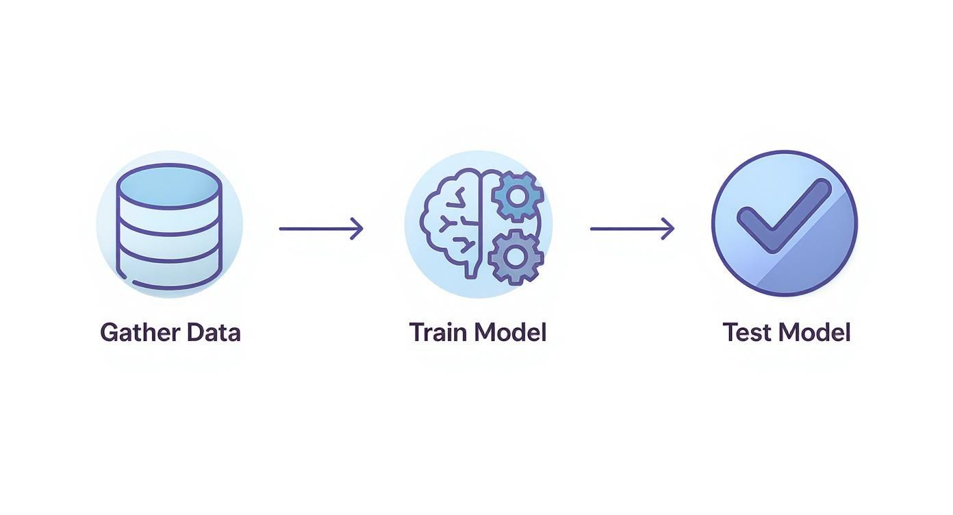
As you can see, it's a linear process where each step builds on the last. It all starts with high-quality data—get that wrong, and nothing else matters.
To bring this process to life, we rely on some powerful tools. Here are the main components you'll be working with:
- Datasets: This is the raw material. It could be a folder with thousands of cat photos, a spreadsheet of stock market data, or transcripts of customer service calls.
- Frameworks: These are libraries like TensorFlow or PyTorch that give you the pre-built components for creating and training networks. You can learn more by checking out our guide on popular machine learning frameworks.
- Hardware: Training is computationally hungry. That's why GPUs (Graphics Processing Units) have become the workhorses of the AI world, capable of handling the massive parallel calculations required.
To get a clearer sense of the road ahead, let's break down the main phases of the training process.
The Core Stages of Neural Network Training
| Stage | What It Means | Why It's Critical |
|---|---|---|
| Data Preparation | Cleaning, labeling, and splitting your raw data into training, validation, and test sets. | Garbage in, garbage out. The model's performance is capped by the quality of its training data. |
| Model Building | Defining the neural network's architecture: choosing layers, neurons, and activation functions. | This is the blueprint for your model. A poor design won't be able to learn the patterns effectively. |
| Training Loop | Feeding data to the model, calculating loss, and using backpropagation to update the model's weights. | This is the "learning" part. The model iteratively adjusts itself to minimize errors and get better at its task. |
| Evaluation | Testing the trained model on unseen data to measure its real-world performance. | This tells you if the model actually learned general patterns or just memorized the training examples. |
These stages form a cycle. You'll often go back and tweak your data or model architecture based on your evaluation results before training again.
My Two Cents: I'll say it again: the single most important factor in any neural network project is the quality of your data. A simple model fed with excellent data will beat a super-complex model with mediocre data almost every time. Plan on spending 80% of your time just getting the data right. It pays the biggest dividends, period.
Getting Your Data Ready for Prime Time
You’ve probably heard the old saying, "garbage in, garbage out," and in machine learning, it’s the absolute golden rule. A brilliantly designed neural network is completely useless if you feed it messy, low-quality data. Getting this first step right is non-negotiable, so let's walk through how to do it.

Think of it like a chef prepping ingredients before cooking. You wouldn't just toss unwashed, unchopped vegetables into a pot and expect a five-star meal. We have to do the same for our data—clean it, organize it, and format it so our model can actually learn something useful.
The Foundation: Data Cleaning and Formatting
Let's ground this with a classic example: the famous MNIST dataset of handwritten digits. Each image is a tiny grid of pixels, with each pixel holding a brightness value. Our goal is to train a model to recognize which digit, from 0 to 9, is in each picture.
Before any learning can happen, we have to make sure the data is clean. This means hunting down common problems:
- Missing Values: Imagine a spreadsheet for predicting house prices where the "square footage" column is empty for some houses. We’d need to either remove those rows or fill in the gaps with a sensible default, like the average square footage.
- Corrupted Data: Sometimes files get mangled, or you'll find images that clearly aren't digits. These outliers have to go; otherwise, they'll just confuse the model.
- Consistent Formatting: Every image needs to be the same size (like 28×28 pixels for MNIST) and use the same color format (like grayscale). If your dataset is a mix, you'll have to resize and convert them all to a uniform standard.
While a well-maintained dataset like MNIST has most of this handled for you, this cleaning phase is where you'll spend a huge chunk of your time on real-world projects.
Normalizing Data for a Fair Fight
With clean data in hand, our next job is normalization. This is just a fancy term for scaling all your numbers to a standard range, usually between 0 and 1.
Why is this a big deal? In our digit example, raw pixel values range from 0 (black) to 255 (white). If we feed those numbers directly into the network, the larger values could have a disproportionate impact, essentially shouting over the signals from smaller-valued features. By scaling every pixel value (for instance, dividing each one by 255), we put all features on a level playing field.
Expert Take: Normalization isn't just a "nice-to-have" step; it's critical for stable and efficient training. It helps optimization algorithms, like gradient descent, find a solution much more smoothly. Without it, your model’s learning can be erratic, taking far longer to converge or even failing to learn anything meaningful at all.
The Crucial Three-Way Data Split
This might be the single most important concept in data preparation. You never train and test your model on the same data. It’s like giving a student the exam questions and the answer key beforehand. Sure, they'll ace the test, but you'll have no idea if they actually learned the material.
To get a true measure of performance, we split our dataset into three independent sets:
- Training Set (Typically 70-80%): This is the bulk of the data. The model churns through this set over and over to learn the underlying patterns.
- Validation Set (Typically 10-15%): We use this set to tune the model during training. After each training cycle (or 'epoch'), we check the model's performance on the validation data. It’s an unbiased report card that helps us make decisions, like when to stop training to avoid overfitting.
- Test Set (Typically 10-15%): This is the final exam. The model never sees this data during training or tuning. Once everything is done, we use this set one time to get an honest, final grade on how well it will perform on new data out in the wild.
Here’s a quick look at how you could do this in Python using the fantastic Scikit-learn library.
from sklearn.model_selection import train_test_split

# Assume X has your images and y has the labels (0-9)
# First, carve out a separate test set
X_train_val, X_test, y_train_val, y_test = train_test_split(X, y, test_size=0.15, random_state=42)

# Now, split the remaining data into training and validation sets
X_train, X_val, y_train, y_val = train_test_split(X_train_val, y_train_val, test_size=0.1, random_state=42)
By meticulously cleaning, normalizing, and splitting your data, you're not just feeding your model—you're setting it up for success from the very beginning. This foundational work is the unsung hero of every high-performing neural network.
Building Your First Neural Network Architecture
Okay, your data is prepped and ready to go. Now for the fun part: designing the brain of your operation. This is where you switch hats from data janitor to architect, sketching out the blueprint for how your model will actually learn.
We'll be using TensorFlow with its Keras API. It’s a fantastic framework for beginners because it lets you turn abstract ideas into functional code without a huge amount of boilerplate.
Think of building a neural network like stacking LEGOs. Each brick is a layer, and the way you arrange them determines what your final creation can actually do. For most beginner projects, the most common and useful brick is the Dense layer. In a Dense layer, every single neuron is connected to every neuron in the previous layer.
Of course, these layers are just the structure. The real "thinking" comes from activation functions. An activation function is a tiny piece of math attached to each neuron that decides whether it should "fire" and pass a signal to the next layer. It's essentially the neuron's on/off switch.
Choosing Your Core Building Blocks
When you're starting out, you don't need a dozen complicated layers. Keep it simple. Two main activation functions will cover most of what you need at first:
- ReLU (Rectified Linear Unit): This is the workhorse for most hidden layers (the ones sandwiched between your input and output). It's super efficient and works by simply passing on the input value if it's positive, and outputting zero otherwise.
- Sigmoid or Softmax: These are usually reserved for the final output layer. Sigmoid is your go-to for binary (yes/no) classification, as it squashes the output to a value between 0 and 1, which you can interpret as a probability. Softmax is for multi-class problems (like our digit recognizer), giving you a probability for each possible class.
Getting deep networks to train effectively used to be a massive headache. The field really took off after 2006, when breakthroughs shifted us toward the deep learning architectures we know today. Before that, deep models were plagued by issues like vanishing gradients. But thanks to new pre-training techniques and huge leaps in GPU power by 2011, models like AlexNet were able to demolish the ImageNet challenge, slashing error rates from 26% down to 15.3%. This proved that deep, end-to-end training wasn't just possible—it was incredibly powerful. You can read more about the history of these deep learning breakthroughs on people.idsia.ch.
A Practical Example: Building a Digit Classifier
Let's build a simple network to classify those handwritten digits from the MNIST dataset. Our images are 28×28 pixels. We'll start by flattening them into a single line of 784 pixels to feed into our first layer.
import tensorflow as tf
from tensorflow.keras.models import Sequential
from tensorflow.keras.layers import Dense, Flatten

# Define the model architecture
model = Sequential([
    # Flatten the 28x28 images into a 784-dimensional vector
    Flatten(input_shape=(28, 28)),

    # First hidden layer with 128 neurons and ReLU activation
    Dense(128, activation='relu'),

    # Output layer with 10 neurons (one for each digit 0-9) and softmax activation
    Dense(10, activation='softmax')
])
This simple structure is a fantastic starting point. It has an input layer to flatten the data, one hidden layer to find patterns, and an output layer to make the final prediction.
My Personal Tip: When you're just starting, resist the urge to build a massive, 20-layer deep network. Start small with one or two hidden layers. As for the number of neurons, using a power of 2 (like 64, 128, or 256) is a common convention, but not a strict rule. You'd be surprised how many problems you can solve with a simple architecture, and it will train much faster, giving you quicker feedback. There are all kinds of ways to structure these layers; you can learn more about the common types of neural network architecture in our guide.
Compiling the Model: Connecting the Pillars of Training
Once the architecture is defined, we need to "compile" it. This step locks in three critical components that will guide the training process.
- Optimizer: This is the engine that updates the model's internal weights to minimize mistakes. 'Adam' is a fantastic, all-around choice. It intelligently adapts the learning rate during training, which often helps you get to a good result faster.
- Loss Function: This tells the model how to measure its own errors. For a multi-class problem like ours, 'sparse_categorical_crossentropy' is the right tool for the job. If we were doing a simple yes/no prediction, we'd use something like 'binary_crossentropy'.
- Metrics: These are the human-friendly scores you'll want to watch. We obviously care about 'accuracy'—the percentage of digits our model identifies correctly.
Here’s how we put it all together in code:
model.compile(optimizer='adam',
              loss='sparse_categorical_crossentropy',
              metrics=['accuracy'])
And that's it! You've just designed and configured your first neural network. This compiled model is now primed and ready for the main event: the training loop, where it will finally start learning from your data.
Running The Core Training Loop
Alright, your data is prepped, and you’ve laid out the blueprint for your model. Now for the main event—the part where the real learning happens. We're about to fire up the training loop, which is the engine that transforms your model from a clueless collection of random weights into a smart, pattern-spotting machine.

This process might sound complex, but modern tools like Keras have made it incredibly straightforward, often just a single line of code. But don't let that simplicity fool you; a lot is going on under the hood, and understanding it is what separates the dabblers from the real practitioners.
Epochs and Batches: The Rhythm of Learning
Before we hit "go," let's quickly nail down two terms you’ll hear constantly when training a neural network: epochs and batch size.
- An epoch is one complete pass through your entire training dataset. If you have 10,000 images, one epoch means the model has seen every single one of them once.
- The batch size is how many examples the model processes before it updates its internal weights. Instead of feeding it all 10,000 images at once (which would be computationally massive), we break them into smaller chunks, or "batches"—say, 32 images at a time.
I like to think of it like studying for a big exam using a huge textbook. An epoch is like reading the entire book from cover to cover. The batch size is how many pages you read before you pause to reflect on what you just learned and tweak your understanding.
A Note From Experience: Choosing the right batch size is more art than science. A batch size of 32 is a classic, safe starting point for most projects. If you have a powerful GPU, larger sizes like 64 or 128 can sometimes speed things up. On the flip side, smaller batches introduce more noise into the training process, which can occasionally help a model escape a rut and find a better solution.
The Three-Step Dance of Learning
When you call a command like model.fit(), you’re essentially kicking off a repetitive, three-step dance that happens over and over for every single batch of data. This cycle is the absolute core of how a neural network learns.
- Forward Propagation (The Guess): The model takes a batch of data—like 32 images of handwritten digits—and passes it forward through its layers. Each layer does its thing, passing the result to the next, until the final layer spits out a prediction for each image.
- Loss Calculation (The Grade): Next, the model compares its predictions to the actual, correct labels using the loss function you chose. This comparison produces a single number, the "loss," which is just a score of how wrong the model was for that batch. A high loss means big mistakes; a low loss means it’s getting warm.
- Backpropagation (The Correction): This is where the magic happens. Using that loss score, the model works its way backward through the network. It calculates how much each individual weight contributed to the total error and nudges it in the right direction to make the error smaller next time.
This constant cycle of guessing, grading, and correcting is how the model slowly but surely gets better. Think of a hiker trying to get down a mountain in a thick fog. They can't see the bottom, so at every step, they feel around for the steepest downward slope and take a small step in that direction. That’s essentially what the model is doing—adjusting its weights in the direction that causes the loss to drop the fastest.
This fundamental process of backpropagation and gradient descent has been the powerhouse behind machine learning breakthroughs for years, enabling models like AlexNet back in 2012 to tune its 60 million parameters.
Visualizing Your Model's Progress
Staring at a stream of updating loss numbers on your screen isn't the most intuitive way to track progress. The single best thing you can do is visualize how your model is learning over time. Two charts are absolutely essential here:
- The Loss Curve: This plots your training loss and validation loss over each epoch. What you want to see is both lines trending steadily downwards.
- The Accuracy Curve: This chart does the same for training and validation accuracy. Here, you want to see both lines climbing upwards.
These charts are your command center. If you see the training loss dropping nicely but the validation loss starts to flatten out or even creep up, you've got a classic case of overfitting. Your model is just memorizing the training data, not learning the underlying patterns. On the other hand, if neither curve improves much, you might be underfitting—the model is too simple for the job.
This visual feedback is non-negotiable for debugging your model and figuring out your next move. The behavior of these curves is heavily influenced by the components inside your network, so if you're curious about what drives these decisions, it's worth understanding the role of activation functions in a neural network.
Is Your Model Actually Any Good? Evaluation and Pitfalls
Alright, you've made it through the training loop, and your loss curve is heading in the right direction. That's a huge step! But now we have to ask the most important question: does the model actually work? This is where we move from training to evaluation—the part of the process that separates a model that just looks good on paper from one that can deliver real-world results.
This is also where we start talking about troubleshooting. Don't worry, every single person who has trained a model has run into these issues.
https://www.youtube.com/embed/LbX4X71-TFI
To get a truly honest assessment, we need to bring out the test set. This is the slice of data your model has never, ever seen. Think of it as the final exam. Its performance here gives you the clearest picture of how it will behave when faced with brand-new, unseen information.
Accuracy Isn't the Whole Story
The first metric everyone looks at is accuracy—the raw percentage of correct predictions. It’s a decent starting point, but it can be dangerously misleading.
Imagine you're building a classifier to detect a rare medical condition that only affects 1% of the population. A lazy model could simply predict "no condition" for every single person and walk away with 99% accuracy. Statistically, it's a success, but in reality, it's completely useless.
This is why we need to dig deeper, especially for classification problems.
- Precision: When the model predicts "yes," how often is it correct? High precision is critical when a false positive is costly. Think of a spam filter: you'd much rather a single spam email slip into your inbox than have a critical job offer flagged as junk.
- Recall: Of all the actual positive cases, how many did the model catch? High recall is essential when a false negative is a disaster. For that rare medical condition, you absolutely need to identify every person who has it, even if it means a few healthy people get flagged for a follow-up test.
Getting a feel for the trade-off between precision and recall is what separates a novice from an experienced practitioner. It's about building a model that solves the actual problem, not just one that gets a high score.
The Beginner's Biggest Hurdle: Overfitting
Let's talk about the single most common trap everyone falls into when they start training neural networks: overfitting. This is what happens when your model gets a little too smart for its own good. It doesn't just learn the underlying patterns in your training data; it starts memorizing the specific examples, noise and all.
You'll know you're overfitting when your training accuracy soars towards 100%, but your validation accuracy hits a wall or even starts to drop. The model has basically memorized the answers to the homework but has no idea how to generalize that knowledge to the final exam.
My two cents: Overfitting isn't a failure; it's a sign that your model is powerful enough to learn. The art is in taming it. Your goal is to dial back the model's complexity just enough so it learns the signal without memorizing the noise.
One of the most effective ways to fight overfitting is Dropout. It's a surprisingly simple idea: during each training update, you randomly "switch off" a fraction of the neurons in a layer. This prevents any one neuron from becoming overly reliant on a specific input feature and forces the network to learn more robust, distributed representations.
What to Do When Things Go Wrong
While overfitting is enemy number one, other issues can pop up.
Sometimes you'll face the opposite problem: underfitting. This is when your model is too simple to capture the underlying patterns in the data. You’ll see both your training and validation accuracy stay disappointingly low. The fix is usually to increase your model's capacity—try adding more layers or more neurons per layer.
Another common frustration is hitting a performance plateau. Your loss curve goes flat after just a few epochs, and learning grinds to a halt. This often points to a problem with your learning rate. If it's too small, your model is taking tiny, inefficient steps. If it's too large, it's bouncing around chaotically and overshooting the optimal solution. Tweaking the learning rate is almost always the first thing I do when I see my model's performance flatline.
Common Questions You'll Have When Training a Neural Network
Even with a perfect plan, you're going to hit some snags. That's just part of the process. Let's walk through some of the most common questions that pop up when you're just getting your hands dirty with neural networks. These are the things that often trip people up at the start.
How Much Data Do I Actually Need?
This is the classic "it depends" question, but I can give you some solid rules of thumb. The amount of data you need is always a function of how complex your problem is.
- Simple Stuff: For a classic task like classifying the MNIST handwritten digits, a dataset with around 50,000 to 60,000 examples will get you to a really high accuracy.
- The Big Leagues: If you're trying to build a massive language model or a high-res image generator from the ground up, you're talking about datasets with billions of data points. For perspective, the Llama 3.1 405B model was trained on a mind-boggling 15 trillion tokens of text.
For most projects you'll start with, a few thousand well-labeled examples for each category you're trying to predict is a good baseline. If you're short on data, don't worry. Transfer learning is your best friend—you can take a model that's already been trained on a huge dataset and just fine-tune it with your smaller, specific one. It's way more efficient.
Why Is My Training So Slow?
Staring at a progress bar for hours can be maddening. If your training is taking forever, it usually comes down to a couple of usual suspects.
The biggest bottleneck is almost always your hardware. Training on a regular CPU (Central Processing Unit) is painfully slow compared to using a GPU (Graphics Processing Unit). GPUs are built to handle thousands of calculations at once, which is exactly what a neural network needs.
My Two Cents: If you're serious about this, get access to a GPU. Whether you buy one or use a cloud service, the speed-up is incredible. It’s not just a small boost; it’s the difference between waiting minutes instead of hours, or hours instead of days.
Your batch size could also be the problem. If it's too small, you're not making full use of your hardware's power with each step. But if it's too big, you might run out of GPU memory, which either crashes the process or forces your system to use much slower memory. It's a balancing act.
Can I Train a Neural Network on My Laptop?
Yes, absolutely! For learning the ropes and tackling smaller projects, your laptop is a great starting point. You can definitely train models for things like basic image classification, text sentiment analysis, or making predictions on structured data.
Modern laptops, especially ones with a dedicated NVIDIA GPU, can handle more than you'd think. Frameworks like TensorFlow and PyTorch run just fine on consumer-grade hardware. No, you won't be training the next big thing on your personal computer, but you can 100% master the fundamentals and build some really cool, practical models. The trick is just to match the project's scope to what your machine can handle.
At YourAI2Day, our goal is to make AI understandable for everyone. We create clear, practical guides to help you build real skills and stay in the loop. To keep learning, check out more articles and resources at https://www.yourai2day.com.