What is Manhattan Distance: Unlocking AI Insights

You’re probably here because you saw Manhattan distance in a machine learning tutorial, a clustering notebook, or a KNN parameter list and thought, “Why would anyone measure distance like a taxi?”

That reaction makes sense. Most of us grow up thinking distance means the shortest straight line between two points. In school, that’s the normal answer. In AI, though, the “normal” answer isn’t always the most useful one.

That’s where this concept gets interesting. What looks like a simple city-block trick turns out to be a practical way to compare data when straight-line geometry stops matching the true structure of the problem. If your data behaves more like streets, grids, counts, independent features, or sparse vectors than smooth physical space, Manhattan distance often feels less weird and more obvious.

Your Guide to Navigating the City of Data

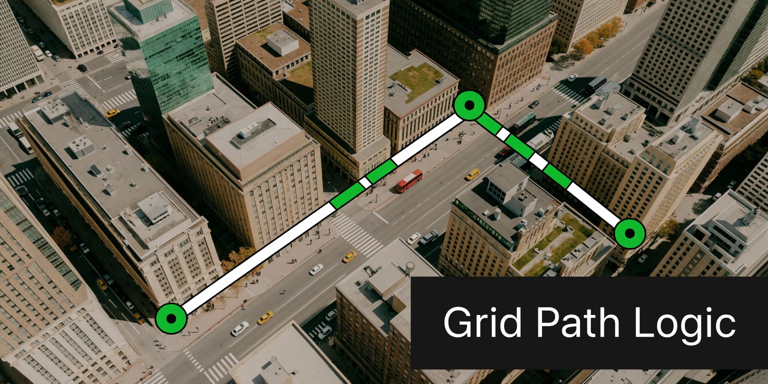
You land in Manhattan, drop your bags at the hotel, and head out for pizza. The shop is a few blocks east and a few blocks north.

You can see the location on the map, but you can’t walk through buildings. You have to follow the streets. So your trip isn’t one straight diagonal line. It’s a sequence of block-by-block moves.

That’s the core idea behind what is manhattan distance. It measures how far apart two points are when movement happens along a grid.

In city terms, you count how many blocks you go left or right, then how many blocks you go up or down, and add them together. That total is the distance.

This sounds almost too simple. But simple is exactly why it matters.

A lot of AI data behaves less like open space and more like a city grid. Think about:

• Text data: A document may contain some words and not others.
• Recommendation systems: A user may like one group of products and ignore another.
• Medical features: A patient profile can include many separate measurements.
• Images and sensor data: Some comparisons work better when each feature contributes directly.

Practical rule: If your features act like separate steps along different streets, Manhattan distance often gives a more useful notion of “closeness” than a straight-line measure.

As a data scientist, I like Manhattan distance because it forces you to ask a better question. Not “what distance formula did I learn first?” but “how does movement happen in this data?”

That shift in thinking matters. It’s the difference between using a default and choosing a metric that matches the structure of the problem.

The Manhattan Distance Formula and Intuition

Manhattan distance, also called L1 distance or taxicab distance, is defined as the sum of the absolute differences of the coordinates. For 2D points (P=(x₁, y₁)) and (Q=(x₂, y₂)), the formula is D(P, Q) = |x₁ – x₂| + |y₁ – y₂|. NIST also notes that this name was popularized through Hermann Minkowski’s early 20th century geometry work, where it corresponds to the L_p norm with p=1 (NIST reference).

Reading the formula like a walk through a city

The formula looks more technical than it really is.

Break it into plain English:

• |x₁ – x₂| means how far apart the points are horizontally
• |y₁ – y₂| means how far apart they are vertically
• Add those two values, and you get the total number of blocks traveled

The absolute value bars matter because distance can’t be negative. If one point is to the left of the other, you still want the positive number of blocks between them.

If absolute values feel rusty, a quick refresher on absolute value equations can help connect the math symbol to the “distance from zero” idea that’s doing the work here.

A concrete 2D example

Take two points:

• P = (1, 2)
• Q = (4, 0)

Now compute the Manhattan distance:

• Horizontal difference: |1 – 4| = 3
• Vertical difference: |2 – 0| = 2
• Total distance: 3 + 2 = 5

So the Manhattan distance is 5.

You can picture that as moving 3 blocks in one direction and 2 blocks in the other.

Where beginners usually get confused

The biggest confusion is this: people think the formula describes one specific path.

It doesn’t.

If you go east first and then south, or south first and then east, the total is still the same. Manhattan distance measures the total required movement along the grid, not the exact route order.

Another common question is whether this works only in 2D. It doesn’t.

The same idea in higher dimensions

In AI, each dimension is just another feature.

If your data point has many features, Manhattan distance adds the absolute difference along every feature. So instead of just horizontal and vertical movement, you’re summing movement across feature 1, feature 2, feature 3, and so on.

That makes it a natural fit for machine learning datasets where each column represents a separate attribute.

Think of each feature as its own street. Manhattan distance asks, “How much total movement do I need across all of them?”

That’s why the formula feels so intuitive once you stop treating it like geometry homework. It’s just accounting for all the feature-by-feature differences directly.

Manhattan vs Euclidean Distance The Grid vs The Bird

The easiest way to compare these metrics is to compare two travelers.

One is a taxi moving through city blocks. The other is a bird flying straight from point A to point B.

Both are measuring distance. They’re just answering different versions of the question.

The core difference

Euclidean distance measures the straight-line path.

Manhattan distance measures the total horizontal and vertical movement.

That’s the geometry difference. The practical difference is even more important.

Euclidean distance squares differences before combining them. Manhattan distance uses absolute differences directly. That means Euclidean tends to punish big deviations more heavily, while Manhattan treats each feature’s contribution more linearly.

Why that matters in data

Suppose two customer profiles differ slightly on many features and differ a lot on one feature.

With Euclidean distance, that one large difference can dominate because of the squaring step.

With Manhattan distance, the same feature still matters, but it doesn’t explode in influence the same way.

That’s one reason many practitioners see Manhattan distance as more stable when data includes irregular values, sparse features, or dimensions with uneven behavior.

Comparison table

Property	Manhattan Distance (L1 Norm)	Euclidean Distance (L2 Norm)
Path idea	Moves along grid directions	Moves in a straight line
Formula style	Sum of absolute differences	Square root of squared differences
Sensitivity to large deviations	Lower	Higher because differences are squared
Best intuitive analogy	Taxi on city streets	Bird flying directly
Behavior in sparse high-dimensional data	Often strong	Can become less informative
Rotation sensitivity	Depends on axis orientation	Less affected by rotation

The “normal” metric isn’t always the better one

A lot of beginners assume Euclidean is more correct because it matches physical intuition.

That’s true for physical space. It’s not automatically true for feature space.

If your data columns represent independent counts, presence or absence, or separate measured attributes, the straight-line shortcut may not reflect how difference should be accumulated. In those settings, adding feature-by-feature differences can be more faithful.

Research summarized by GeeksforGeeks reports that in high-dimensional AI applications, Manhattan distance often outperforms Euclidean distance on sparse data, with k-NN on Iris reaching 95-98% accuracy versus 92-95% for Euclidean because L1 helps mitigate the curse of dimensionality (GeeksforGeeks).

A subtle trade-off practitioners should know

Manhattan distance depends more on the coordinate axes you choose.

If you rotate the feature space, Manhattan distances can change in a way Euclidean distances don’t. That sounds abstract, but in practice it means feature engineering matters. If your columns have a strong axis-aligned meaning, such as counts per category or independent measurements, Manhattan often makes good sense. If your problem is naturally geometric and orientation-independent, Euclidean may fit better.

Use Euclidean when straight-line geometry is the story. Use Manhattan when total coordinate-wise change is the story.

That’s the key comparison. Not which metric is universally better, but which one matches how difference should behave in your data.

Manhattan Distance in Practice Code and Numeric Examples

A formula only becomes useful when you can work with it quickly. So let’s do one hand calculation, then turn it into Python.

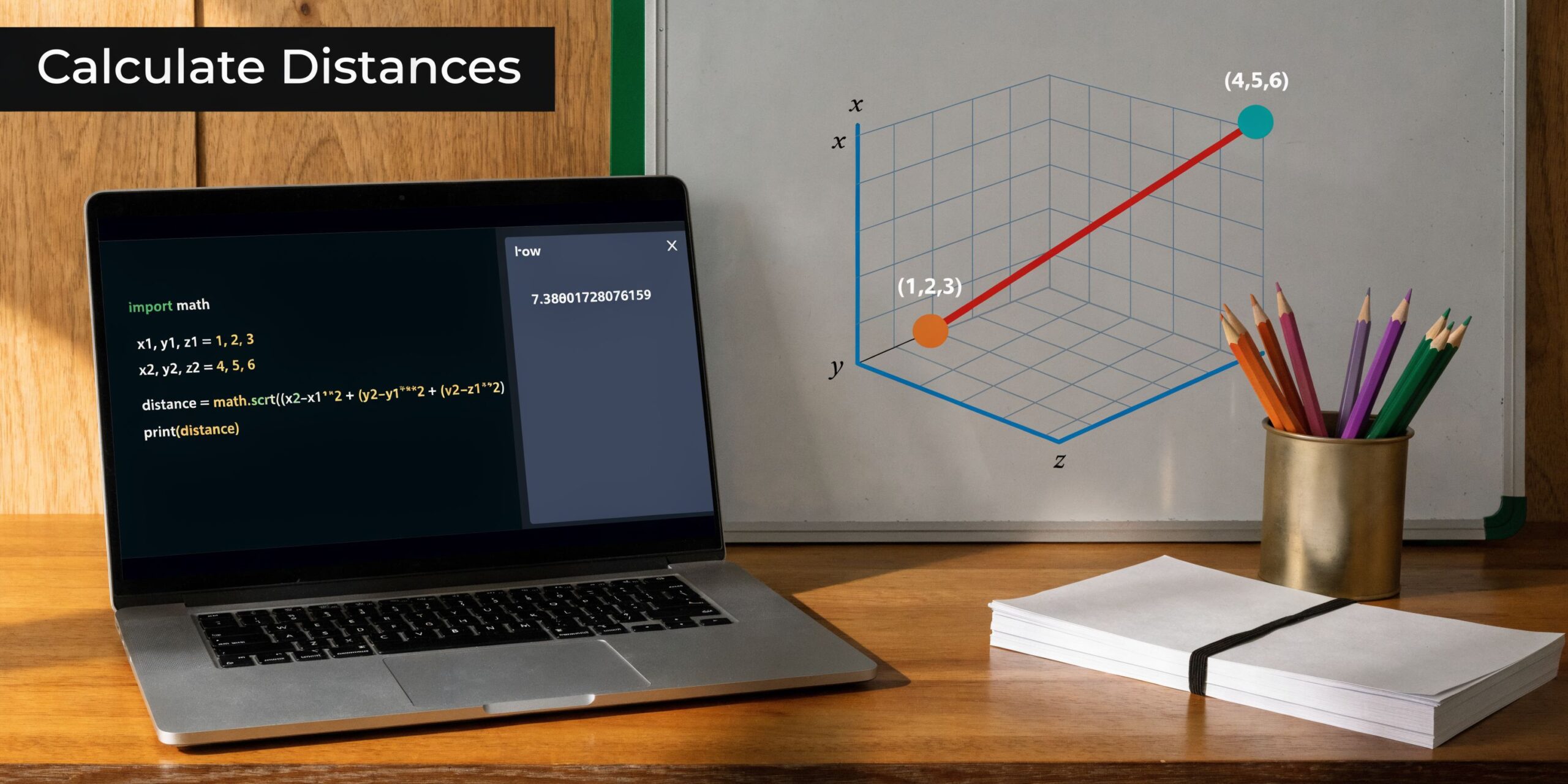
A simple 3D example

Take these two vectors:

• C = (3, 2, 5)
• D = (4, 1, 7)

For Manhattan distance, calculate the absolute difference in each dimension:

• |3 – 4| = 1
• |2 – 1| = 1
• |5 – 7| = 2

Add them:

• 1 + 1 + 2 = 4

So the Manhattan distance is 4.

For comparison, Euclidean distance for the same vectors is √[(1)² + (1)² + (2)²] = √6 ≈ 2.45, as shown in the AlgoDaily explanation of Manhattan distance in KNN contexts (AlgoDaily).

That difference in output is normal. Manhattan distance often gives a larger value because it follows the grid logic instead of taking a straight shortcut.

Python code you can copy

If you use SciPy, the cleanest option is cityblock().

from scipy.spatial.distance import cityblock
import numpy as np

a = np.array([3, 2, 5])
b = np.array([4, 1, 7])

dist = cityblock(a, b)
print(dist)  # 4

If you want to compute it manually with NumPy, that’s also straightforward:

import numpy as np

a = np.array([3, 2, 5])
b = np.array([4, 1, 7])

dist = np.sum(np.abs(a - b))
print(dist)  # 4

When I’d use each approach

• SciPy cityblock works well when you want a standard library function.
• NumPy with np.abs and np.sum is great for learning and debugging.
• scikit-learn metric settings are what you’ll usually use inside a model pipeline.

If you can explain the result by hand for one small vector pair, you’ll trust the library output more when you scale up.

That’s a good habit for beginners. Metrics feel abstract until you compute one yourself and see that it’s just feature-by-feature difference added up.

Why AI and Machine Learning Love Manhattan Distance

When people ask what is manhattan distance doing in AI, the short answer is this: it gives models a practical way to compare data when features are numerous, sparse, or naturally independent.

That shows up most clearly in K-Nearest Neighbors, where the algorithm depends on distance to decide which examples count as “near.”

KNN is only as good as its distance metric

KNN is simple in spirit. Given a new data point, look for the closest labeled examples and let them vote.

That means the distance metric isn’t a small implementation detail. It defines what “close” means.

If your dataset has lots of dimensions, especially sparse ones, Manhattan distance often behaves better than Euclidean distance. AlgoDaily notes that scipy.spatial.distance.cityblock() computes in O(n) and can be 20-50% faster than Euclidean distance on large samples with many dimensions, and this can improve F1-scores by 5-15% in some classification tasks (AlgoDaily).

Why sparse data changes the game

Think about text classification.

A document vector might have many features, but most of them are zero. That’s a classic sparse setup. In this kind of space, Euclidean distance can become less helpful because many points end up looking similarly far apart. Manhattan distance often preserves a clearer sense of coordinate-by-coordinate difference.

This matters in:

• Document classification
• Recommendation pipelines
• User behavior vectors
• Bag-of-words and count-based representations

If you’re sorting out where this fits in the broader AI stack, this explainer on Deep Learning vs Machine Learning is a useful companion because distance metrics show up most directly in classical ML workflows, even though the ideas still influence modern systems.

The curse of dimensionality in plain English

As dimensions pile up, distance can get weird.

Points that felt clearly near or far in 2D start bunching together in higher dimensions. Euclidean distance is especially vulnerable because the squared terms can blur useful distinctions when many dimensions are involved.

Manhattan distance often holds up better because it keeps adding straightforward per-feature differences. That can make neighborhoods in KNN more meaningful.

If you want a practical implementation example, YourAI2Day has a related KNN walkthrough in R at https://yourai2day.com/k-nearest-neighbor-in-r/.

Beyond KNN

Manhattan distance also shows up in clustering and feature comparison.

In my experience, it’s especially useful when:

1. Features are independent: Each column contributes separately.
2. Zeros are common: Sparse vectors are everywhere in data.
3. Interpretability matters: Summed absolute differences are easier to explain to teams.

Here’s a quick visual refresher before you try it yourself:

Don’t treat distance as a default parameter. In models like KNN, distance is part of the model’s logic.

That’s the big takeaway. Manhattan distance isn’t there to be mathematically different. It’s there because, in many AI tasks, it matches the data better.

Beyond Machine Learning Unexpected Applications

Manhattan distance isn’t just an ML classroom concept. Engineers use it in systems where movement or layout is constrained to horizontal and vertical paths.

Chip design is the clearest example.

Why it matters in VLSI and hardware

In VLSI design, wires on chips run along axis-aligned paths. Engineers don’t route them as free-floating diagonals. They route them like streets on a grid.

That makes Manhattan distance a natural fit for wire-length estimation and routing decisions. NIST’s Dictionary of Algorithms and Data Structures describes this axis-parallel use, and the same reference notes benchmark claims that Manhattan-based routers can reduce via count by 15% and congestion by 20%, helping with power savings and density scaling in modern processors and AI hardware (NIST DADS).

It also shows up in logistics

Urban delivery has the same flavor.

If a vehicle has to follow a city street network, straight-line distance can underestimate the actual travel path. Manhattan distance gives a cleaner first approximation because it respects grid movement.

That’s one reason this metric keeps showing up in operational thinking, not just theory.

A useful mental bridge from text data to chip routing

These use cases look unrelated at first.

One is digital text or recommendation data. The other is physical hardware routing. But the underlying pattern is the same: you aren’t moving freely in all directions. You’re moving through constrained steps.

That’s also why sparse text representations pair so naturally with matrix-style tools like a https://yourai2day.com/term-document-matrix/. Both cases reward thinking in coordinate-wise differences rather than smooth geometric shortcuts.

Good metrics come from constraints. Manhattan distance works well when the world, or the data, makes you move one axis at a time.

That’s the deeper lesson. This isn’t an “AI trick.” It’s a way to model problems accurately.

Choosing Your Metric A Practical Decision Guide

When you’re building a model, metric choice should follow the data, not habit.

I wouldn’t treat Manhattan distance as the answer to everything. I would treat it as one of the first options to test when the data has a grid-like or sparse structure.

Use Manhattan distance when

These are the situations where L1 usually deserves serious consideration:

• Your data is sparse: Text vectors, event counts, and many recommendation features fit this pattern.
• Features act independently: You want each column to contribute directly to total difference.
• You prefer stability: Absolute differences avoid the stronger penalty that Euclidean gives to large deviations.
• You’re working in many dimensions: A YouTube-based analysis cited in the verified data reports that in cases with over 50 dimensions, Manhattan distance was preferred in 65% of ML pipelines analyzed and boosted KNN precision by 18% on sparse e-commerce data (YouTube reference).

Use Euclidean distance when

Euclidean still makes sense in plenty of settings:

• Physical space or geometry matters.
• Straight-line closeness reflects the true problem.
• Your features behave more like coordinates in continuous space than independent counts.

Don’t ignore preprocessing

A distance metric can only work with the feature space you hand it.

If one feature has a much larger numeric scale than others, it can dominate either metric. So scaling, normalization, and sensible feature design still matter. Metric choice doesn’t replace data preparation.

If you’re thinking through model behavior more broadly, it also helps to understand how optimization targets interact with distance-driven decisions. This overview of https://yourai2day.com/loss-function-machine-learning/ is a useful next read.

A quick comparison with Chebyshev distance

There’s also a third metric worth knowing: Chebyshev distance.

Instead of summing differences, it takes the largest absolute difference across dimensions. So if Manhattan asks for total block travel, Chebyshev asks for the single biggest move required on any axis.

That makes it useful in special cases, but for most beginner workflows, the practical choice is still between Manhattan and Euclidean.

My rule-of-thumb checklist

When I’m advising a teammate, I usually ask:

1. Are these features sparse or mostly zero?
2. Do the columns represent separate, additive differences?
3. Would one large deviation unfairly dominate if we squared everything?
4. Are we using KNN or another distance-heavy method?
5. Does the data behave more like a street grid than open space?

If the answers lean yes, Manhattan distance moves way up the shortlist.

Decision shortcut: If your data lives in a “feature city” instead of a smooth geometric field, test Manhattan early.

That’s the key habit to build. Don’t inherit the default. Justify the metric.

The Shortest Path to Understanding

The nicest thing about Manhattan distance is that the intuition never gets lost.

You start with a taxi moving through city blocks. Then you realize that many datasets behave the same way. They don’t reward diagonal shortcuts. They reward counting the total movement across separate features.

That’s why this metric keeps showing up in AI. It’s simple, interpretable, and often better aligned with sparse, high-dimensional data than the straight-line distance many beginners assume must be best.

If you remember only a few ideas, keep these:

• Manhattan distance is the sum of absolute coordinate differences.
• It works well when data behaves like a grid.
• It often shines in KNN and other distance-based workflows with sparse, high-dimensional features.
• It’s also useful beyond ML, including chip routing and urban-style path problems.
• The right metric depends on the structure of the problem, not on what feels most familiar.

Once you see distance metrics this way, model building gets more thoughtful. You stop accepting defaults and start asking whether your metric matches the world your data lives in.

That’s a strong habit for any AI practitioner, especially early on.

---

If you want more plain-English explanations of AI concepts, practical guides, and examples you can use in real projects, explore YourAI2Day. It’s a useful place to keep building intuition around machine learning, tools, and the core ideas that make AI systems work.