Loss Function Machine Learning: A Practical Guide to Boost Your AI Models

At its core, a loss function in machine learning is the component that tells a model how far off its predictions are from the actual truth. Think of it as a penalty score. A high score means the model's guess was way off, while a low score indicates it's getting warm.

This single number is the most critical piece of feedback a model gets. It’s the driving force behind how it learns and gets better.

The Heartbeat of AI Training

Let's get practical. Say you're training an AI to recognize photos of cats. You show it a picture of a fluffy Persian, and it responds, "I'm 70% confident this is a cat." Since you know for a fact it's a cat, the right answer is 100%. The loss function steps in to measure that 30% gap. It calculates the "error" or "loss" from that one guess.

But this loss value isn't just a grade—it's a roadmap. It gives the model the exact information it needs to tweak its internal settings, aiming to be just a little bit more accurate next time. The whole training process is just a continuous loop: guess, measure the error, and adjust to lower that error.

The Score That Drives Learning

Using a number to measure and correct mistakes isn't a new idea. The journey from early statistical error theory to today's machine learning frameworks represents a massive evolution in computational learning. While early ideas about error were often theoretical, the development of backpropagation in the 1980s was a game-changer. It gave machines a practical way to use these error scores to systematically improve. You can dive deeper into the history and evolution of error correction in learning.

Today, this simple loop is the engine that powers almost all of modern AI. Every time a model trains, it's essentially playing a game of "get the loss score as close to zero as possible."

Expert Opinion: I like to think of the loss function as the model's conscience. It's that little voice whispering, "Nope, that wasn't quite right. Try again, but adjust this way." Without it, a model is just guessing in the dark. It’s the crucial link between making a prediction and actually learning something.

Why Is It Called a "Loss"?

The term "loss" is quite intuitive. It represents the information that is "lost" when a model's prediction doesn't perfectly align with the ground truth. A model that makes flawless predictions would have a loss of zero.

Of course, perfection is rare. The real goal is to minimize this value—to get it as close to zero as we can. This simple, singular objective is what makes the loss function a machine learning cornerstone.

How a Loss Score Teaches Your AI to Improve

So, your AI model made a guess and the loss function slapped it with a penalty score. What’s next? That score isn't just a report card; it's the kick-off for the entire learning process. This is the moment the model stops just guessing and starts intelligently improving.

Think of a hiker lost in a thick, foggy valley. Their goal is to find the lowest point, but they can only see a few feet ahead. The loss score is their altimeter—it tells them their current elevation. A high score means they're way up on a steep hill (a big mistake), while a low score means they're getting closer to the valley floor (the minimum error).

Introducing Gradient Descent: Your AI's Compass

Knowing your elevation is one thing, but it doesn't tell you which way to walk. To find the path down, our hiker needs a compass. In machine learning, that compass is a mathematical tool called a gradient.

The gradient is just a fancy word for the slope of the loss function right where the model is currently "standing." It points in the direction of the steepest ascent—straight uphill. Since our goal is to minimize the loss, we just flip that direction around.

By taking a small step in the opposite direction of the gradient, our model is guaranteed to be moving downhill, getting a little closer to that sweet spot of minimum error.

This whole cycle—calculating the loss, finding the gradient, and taking a small step downhill—is called Gradient Descent. It's the engine that drives training for most neural networks and machine learning models today.

Expert Opinion: Gradient Descent is the workhorse of deep learning. It's an elegant and surprisingly effective way to navigate incredibly complex, high-dimensional spaces. The beauty is its simplicity—calculate the slope, take a step downhill, and repeat. Billions of times.

The Learning Rate: Deciding the Size of Each Step

How big of a step should the model take? That's controlled by a critical setting called the learning rate. This parameter dictates how much the model adjusts its internal knobs and dials in response to the error it just saw.

Getting the learning rate right is a bit of an art, and it's absolutely crucial for effective training. Here’s a breakdown of what can happen:

• Learning Rate Too High: Imagine our hiker taking giant, reckless leaps down the mountain. They might overshoot the valley floor entirely and land on the other side, even higher than before! The model's loss score will jump around erratically and might never settle on the lowest point.
• Learning Rate Too Low: Now picture the hiker taking tiny, shuffling steps. They'll get to the bottom eventually, but it's going to take forever. The training process becomes painfully slow and might get stuck in a rut before finding the best solution.

The goal is to find a "Goldilocks" learning rate—not too big, not too small—that allows the model to descend efficiently without becoming unstable. This feedback loop is fundamental to how AI works. It's a key concept to grasp when you're figuring out how to train AI chatbots or any other complex model.

Putting It All Together: The Training Loop

So, how does this all connect in practice? The entire training process boils down to a simple loop that repeats thousands, or even millions, of times.

1. Predict: The model looks at a batch of data (like a set of images) and makes a prediction for each one.
2. Calculate Loss: The loss function compares these predictions to the real answers and spits out a single penalty score.
3. Compute Gradient: The algorithm calculates the gradient of that loss, figuring out the "downhill" direction.
4. Update: The model takes a small step in that direction, tweaking its internal parameters to get just a little bit better.
5. Repeat: The loop starts over with a new batch of data.

With every single cycle, guided by its loss function, the model gets a tiny bit smarter. To go even deeper into this incredible process, you can explore more about how neural networks learn from data and build their own understanding.

Common Loss Functions and When to Use Them

Just like a carpenter wouldn't use a sledgehammer to drive a tiny finishing nail, you can't just pick one loss function and use it for every machine learning problem. The kind of task you're tackling—whether it’s predicting a house price or flagging an email as spam—fundamentally changes the tool you need to measure your model's mistakes.

Choosing the right loss function is one of the most critical decisions you'll make. It’s not just an academic exercise; it directly tells your model what to care about. A loss function's job is to penalize errors, but how it doles out that penalty can completely alter the final result. Some functions react dramatically to big mistakes, while others are more forgiving.

Let's walk through the essential toolkit of loss functions for the two most common machine learning tasks: regression and classification.

Loss Functions for Regression Problems

Regression is all about predicting a continuous number. Think stock prices, temperatures, or home values. The name of the game is getting your prediction as close to the actual number as possible. In this space, two functions are king: Mean Squared Error and Mean Absolute Error.

1. Mean Squared Error (MSE)

Mean Squared Error, or MSE, is the workhorse of regression. The process is simple: it finds the difference between the model's prediction and the true value, squares that difference, and then averages all those squared differences across your dataset.

So, why square the error? This little bit of math does two very important things. First, it makes all errors positive, so you don't have a positive error canceling out a negative one. But more importantly, it massively penalizes larger errors.

A single wildly incorrect prediction can blow up your loss score and yank the model's parameters in a dramatic, unhelpful direction. This is both MSE's biggest feature and its biggest weakness.

Practical Example: House Price Prediction
Imagine your model predicts a house will sell for $350,000, but the actual sale price was $300,000. The error is $50,000. MSE squares this to a staggering 2,500,000,000.

Now, say another prediction is off by just $5,000. Its squared error is only 25,000,000. The first mistake contributes 100 times more to the total loss, forcing the model to fixate on that one big miss. This makes MSE a great choice when large errors are exceptionally damaging and you need your model to avoid them at all costs.

2. Mean Absolute Error (MAE)

Mean Absolute Error (MAE) offers a more straightforward approach. Instead of squaring the difference, it just takes the absolute value. Then, it averages those absolute differences.

With MAE, a $50,000 mistake is simply ten times worse than a $5,000 mistake. There's no dramatic squaring involved, which makes MAE far more robust to outliers. That one wildly incorrect house price prediction won't hijack the entire training process.

• When to use MAE: This is your go-to when your dataset has outliers you don't want the model to obsess over. For example, if you're predicting customer support wait times and a few system outages caused hour-long delays, MAE prevents those extreme cases from warping the entire model.

Loss Functions for Classification Problems

Classification is a different beast entirely. You're not trying to get close to a number; you're trying to pick the right label. Is this email "spam" or "not spam"? Is this image a "cat," "dog," or "bird"? The loss functions here are designed to measure how confident the model was when it picked the wrong answer.

Binary Cross-Entropy Loss

For any problem that boils down to a simple yes-or-no decision (binary classification), Binary Cross-Entropy is the industry standard. It's the loss function machine learning experts rely on for tasks like spam detection, medical diagnoses (e.g., malignant vs. benign tumor), or predicting if a user will click an ad.

It works by looking at the model's predicted probability and comparing it to the actual class (0 or 1). If the model gives a high probability to the correct class, the loss is tiny. But if it gives a high probability to the wrong class, the loss skyrockets.

Practical Example: Spam Email Detection
Let's say a known spam email arrives (actual class = 1).

• If your model predicts there's a 95% chance it's spam, the cross-entropy loss is very small. The model did a great job.
• But if your model predicts there's only a 5% chance it's spam (meaning it was 95% sure it was not spam), the loss will be huge. The model wasn't just wrong; it was confidently wrong, and cross-entropy punishes that severely.

Quick Guide to Common Loss Functions

Choosing a loss function can feel daunting, but you'll find that a few core options cover most of the problems you'll encounter. Here's a quick cheat sheet to help you match the right function to your task.

Loss Function	Problem Type	Best For	Key Trait
Mean Squared Error (MSE)	Regression	When large errors are especially bad.	Squares errors, heavily penalizing outliers.
Mean Absolute Error (MAE)	Regression	Datasets with significant outliers.	More robust and less sensitive to outliers.
Binary Cross-Entropy	Binary Classification	"Yes/No" or "0/1" predictions.	Punishes confident but incorrect predictions.
Categorical Cross-Entropy	Multi-Class Classification	When an item belongs to only one of many categories.	Ideal for "cat vs. dog vs. bird" problems.
Hinge Loss	Classification	Primarily used with Support Vector Machines (SVMs).	Focuses on getting the classification "right enough."

This table is just a starting point, but it covers the foundational tools you'll need for most supervised learning challenges.

Ultimately, loss functions are the measurement systems that tell your model how well it's doing. Functions with smooth gradients, like MSE and Cross-Entropy, often lead to faster, more stable training. In regression, MSE has long been the default, but it's important to recognize the trade-offs it introduces. To learn more about these nuances, check out this in-depth guide on loss functions and their properties on datacamp.com.

Picking the right loss function is a fundamental step that aligns your model's training objective with your real-world goal, making sure it learns to minimize the errors that actually matter.

Diving Deeper: More Specialized Loss Functions

While the loss functions we've covered are the workhorses for most day-to-day regression and classification jobs, the machine learning world is full of unique problems. To tackle them, data scientists have cooked up some pretty specialized tools. Let's peel back another layer and look at a few advanced loss functions that drive some of the most impressive AI systems out there.

These aren't just slight tweaks on a theme; they represent fundamentally different ways of framing the problem of error. Instead of just asking, "How wrong was the prediction?" they might ask, "How confident was that mistake?" or "How different is this generated image from a real one?" This is where the creative, problem-solving side of machine learning really comes alive.

Hinge Loss for Maximum Margin Classification

Ever wonder how some models can draw such a clean, confident line between different groups of data? A lot of the time, the secret sauce is Hinge Loss. This is the clever engine behind a classic and powerful model: the Support Vector Machine (SVM).

Unlike cross-entropy, which obsesses over getting the probability scores just right, Hinge Loss is a bit more pragmatic. Its main goal is to find a decision boundary that is not only correct but also has the widest possible "buffer zone" or "margin" separating the classes.

• Its Philosophy: So long as a prediction is on the correct side of this margin, Hinge Loss gives it a pat on the back and assigns a loss of zero. It only starts penalizing the model when a prediction is either flat-out wrong or lands inside that buffer zone, which tells the model it isn't being confident enough.
• Practical Example: Think about a security system classifying people as "authorized" or "unauthorized" from facial scans. Hinge Loss would push the model to create a very clear separation, making the system less likely to get tripped up by someone who just happens to look a little like an authorized person. It’s all about creating a robust, confident boundary.

The evolution of loss functions is one of the biggest tech stories of the last century, completely changing how machines learn. By the 1990s, Support Vector Machines put hinge loss in the spotlight, maximizing the margin between classes and offering a fresh take on classification. This was a massive step, as loss functions became the quantitative backbone that let neural networks improve through gradient descent. You can learn more about how these historical developments shaped modern AI on arxiv.org.

KL Divergence for Generative Models

Alright, let's switch gears and step into the world of generative AI, where models create brand-new things—text, art, music, you name it. How do you possibly measure "error" when there isn't a single correct answer? This is exactly where Kullback-Leibler (KL) Divergence shines.

KL Divergence isn't your typical loss function that compares one prediction to one answer. Instead, it measures how different one probability distribution is from another.

Expert Opinion: Think of KL Divergence as a way of measuring surprise. If your generative model produces a sentence that sounds perfectly natural (matching the distribution of real human language), the KL Divergence is low—no surprise there. But if it spits out nonsensical gibberish, the divergence is high because it’s so wildly different from what we'd expect.

For generative models, the whole point is to create outputs that are statistically indistinguishable from the real-world data they were trained on. KL Divergence is the perfect tool for the job, quantifying how well the model's generated distribution mirrors the target distribution of real data. This concept is at the heart of advanced models like Variational Autoencoders (VAEs) and is critical for tasks like fine-tuning large language models. For those interested in going down that rabbit hole, you might find our guide on how to fine-tune an LLM useful.

These specialized functions prove that a loss function in machine learning is more than a dry formula; it's a declaration of what you want your model to value. By picking the right one, you can guide your AI to not just be accurate, but to be confident, creative, and truly robust.

How to Choose and Apply a Loss Function in Your Code

This is where the theory hits the road. We've talked about what loss functions are, but now it's time to actually pick one and get it working in a real model. The good news? Choosing the right loss function in machine learning isn't some black art. It's a logical process driven by a single, simple question.

What kind of answer are you trying to get from your model? Seriously, that's it. Your answer will immediately narrow the field and point you toward the right family of loss functions.

A Simple Decision Framework

Let's think about your project's goal. Are you predicting a number that can fall anywhere on a continuous scale, like a home price or tomorrow's temperature? Or are you trying to sort things into neat, distinct buckets, like "spam" vs. "not spam"?

We can break this down into three of the most common scenarios you'll encounter:

• Predicting a Continuous Number (Regression): If your goal is to predict a numerical value—think house prices, stock values, or energy consumption—you're doing regression. Your go-to loss functions here will almost always be Mean Squared Error (MSE) or Mean Absolute Error (MAE).
• A "Yes" or "No" Choice (Binary Classification): When the task is to make a simple either/or decision, you're in the world of binary classification. Is this email spam? Will this customer churn? For these jobs, the undisputed champion is Binary Cross-Entropy.
• Sorting Into Multiple Categories (Multi-Class Classification): Need to assign an item to one of several possible groups? For example, classifying news articles into "Sports," "Politics," or "Technology." This is multi-class classification, and you'll want to use Categorical Cross-Entropy.

This initial decision cuts through the noise, taking you from dozens of potential choices to just one or two highly relevant ones. From there, you can get more specific. The flowchart below is a great visual guide for when you need to move beyond the basics and into more specialized functions.

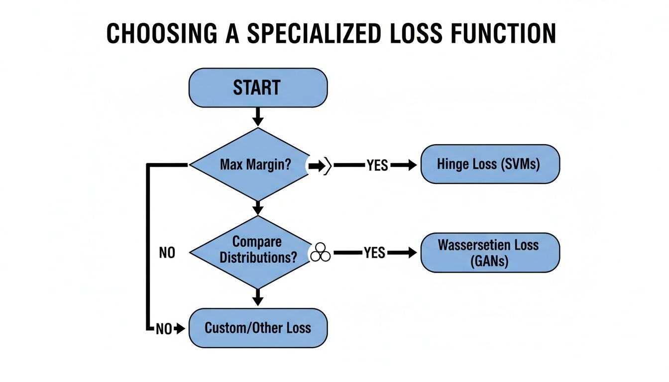
As you can see, once you know your goal—whether it's creating a clear buffer between classes or generating new data that looks real—the path to the right advanced loss function becomes much clearer.

From Concept to Code

Here’s the best part: modern frameworks like PyTorch and TensorFlow have made putting a loss function into your code ridiculously easy. Most of the time, it's literally a single line.

Just to show you how simple it is, here’s how you would define Binary Cross-Entropy in both frameworks.

In PyTorch:

import torch.nn as nn

# Define the loss function for a binary classification problem
loss_function = nn.BCELoss()

In TensorFlow/Keras:

import tensorflow as tf

# Compile the model, specifying the loss function
model.compile(optimizer='adam',
              loss=tf.keras.losses.BinaryCrossentropy(),
              metrics=['accuracy'])

That’s all there is to it. You pick the pre-built function that matches your problem, and the framework takes care of all the heavy lifting behind the scenes. Of course, the next step is actually using it. If you're ready for that, our guide on how to train a neural network is a great place to start.

Common Mistakes to Avoid

As you get your hands dirty with code, a few common tripwires can cause hours of frustrating debugging. Knowing what they are ahead of time can save you a massive headache.

Expert Opinion: The most frequent mistake I see beginners make is a mismatch between the final layer activation and the loss function. For instance, using a sigmoid activation for multi-class classification or forgetting to apply a softmax before Categorical Cross-Entropy. These small mismatches can prevent your model from learning at all.

Here are two classic blunders to keep on your radar:

1. Wrong Loss for the Wrong Problem: Never, ever use a regression loss like MSE for a classification task. While it's technically possible to make the code run, the model will learn terribly. MSE just isn't built to penalize a model for picking the wrong category.
2. Output Shape Mismatch: Make sure the output from your model's final layer is in the exact format the loss function is expecting. For example, Binary Cross-Entropy needs a single probability value between 0 and 1 for each input. If your model spits out something else, it’s going to break.

By sticking to this simple framework and sidestepping these common errors, you'll be well on your way to choosing and applying the right loss function every time. And when you're ready to deploy, incorporating the top MLOps best practices will ensure your models are managed effectively in production.

Answering Your Burning Questions About Loss Functions

As we start to wrap things up, it's completely normal for a few questions to be rattling around in your head. Loss functions are a deep topic with plenty of nuance, so let’s clear up some of the most common points of confusion. Think of this as the FAQ section to really lock in what you've learned.

What’s the Difference Between a Loss Function and a Metric?

This is a fantastic question, and probably the most common one I hear. While they both measure performance, they're built for two entirely different audiences.

• A loss function is for the machine. Its main job is to give the optimization algorithm—like Gradient Descent—a smooth, continuous signal it can follow to update the model's parameters. The actual value of the loss isn't always something you can easily interpret.

• A metric, on the other hand, is for you. Things like accuracy, precision, or F1-score are designed to tell a human how well the model is actually doing its job in a way that makes sense.

So, you train the model by minimizing the loss, but you report the accuracy to your team. For example, seeing the Binary Cross-Entropy loss drop from 0.12 to 0.08 is kind of abstract. But seeing the accuracy jump from 92% to 95%? That’s a clear win.

Can I Just Make My Own Loss Function?

Absolutely! In fact, creating a custom loss function machine learning solution is a hallmark of more advanced, tailored AI systems. You do this when a standard-issue function doesn't quite capture the unique costs or goals of your specific problem.

Imagine you're predicting inventory needs for a retail business. The cost of understocking (and missing a sale) might be 10 times worse than the cost of overstocking (and having extra product). You can build a custom loss function that penalizes under-predictions way more heavily than over-predictions, directly tying the model's learning process to your real-world financial outcomes.

The one non-negotiable rule is that your custom loss function must be differentiable. The optimizer has to be able to calculate its gradient to know which way to nudge the model's weights. No gradient, no learning.

Help! Why Did My Model’s Loss Stop Decreasing?

Ah, the dreaded plateau. When your loss value flatlines and refuses to budge, it means your model has stopped learning. It's a frustrating but incredibly common rite of passage for anyone building models.

The number one culprit is almost always the learning rate. If it’s too high, the optimizer is like a clumsy giant, stomping around and constantly overshooting the best solution. If it's too low, its steps are so tiny that it’s making no meaningful progress, like trying to cross an ocean by taking microscopic steps.

Other common suspects include:

• Data problems: Your data might not be properly scaled or cleaned, which can make the training process unstable.
• A simplistic model: The model itself might be too simple for the job (underfitting) and just doesn't have the capacity to learn the complex patterns in the data.
• Good old-fashioned bugs: Sometimes, it’s just a simple mistake in your training loop or data pipeline. Never underestimate this one!

Figuring out why a model's loss is stuck is a core skill in machine learning, and it often feels a lot like detective work.

Does a Lower Loss Always Mean a Better Model?

Not necessarily, and this brings us to one of the most critical concepts in all of machine learning: overfitting.

A model can achieve an almost-zero loss on its training data simply by memorizing it. It learns every single data point, including all the random noise and quirks that aren't actually part of the real pattern.

The problem? This "memorized" knowledge doesn't generalize to new situations. When you show the model new, unseen data, it completely falls apart because it never learned the underlying rules. This is exactly why we always hold back a separate validation or test dataset to get an honest measure of performance.

A truly great model isn't the one with the lowest possible training loss. It's the one that achieves a low loss on both the data it trained on and the new data it has never seen before. That balance is the real goal.

---

At YourAI2Day, our goal is to break down complex AI topics into clear, actionable insights. To keep building your skills and stay on top of what’s happening in artificial intelligence, feel free to explore more of our resources.